Tales from the Binomial Tail: Confidence intervals for balanced accuracy

At Groundlight, we put careful thought into measuring the correctness of our machine learning detectors. In the simplest case, this means measuring detector accuracy. But our customers have vastly different performance needs since our platform allows them to train an ML model for nearly any Yes/No visual question-answering task. A single metric like accuracy is unlikely to provide adequate resolution for all such problems. Some customers might care more about false positive mistakes (precision) whereas others might care more about false negatives (recall).

To provide insight for an endless variety of use cases yet still summarize performance with a single number, Groundlight's accuracy details view displays each detector's balanced accuracy. Balanced accuracy is the average of recall for all classes and is Groundlight's preferred summary metric. For binary problems, this is just the mean of accuracy on the should-be-YES images and accuracy on the should-be-NOs. We prefer balanced accuracy because it is easier to understand than metrics like the F1 score or AUROC. And since many commercially interesting problems are highly imbalanced - that is the answer is almost always YES or always NO - standard accuracy is not a useful performance measure because always predicting the most common class will yield high accuracy but be useless in practice.

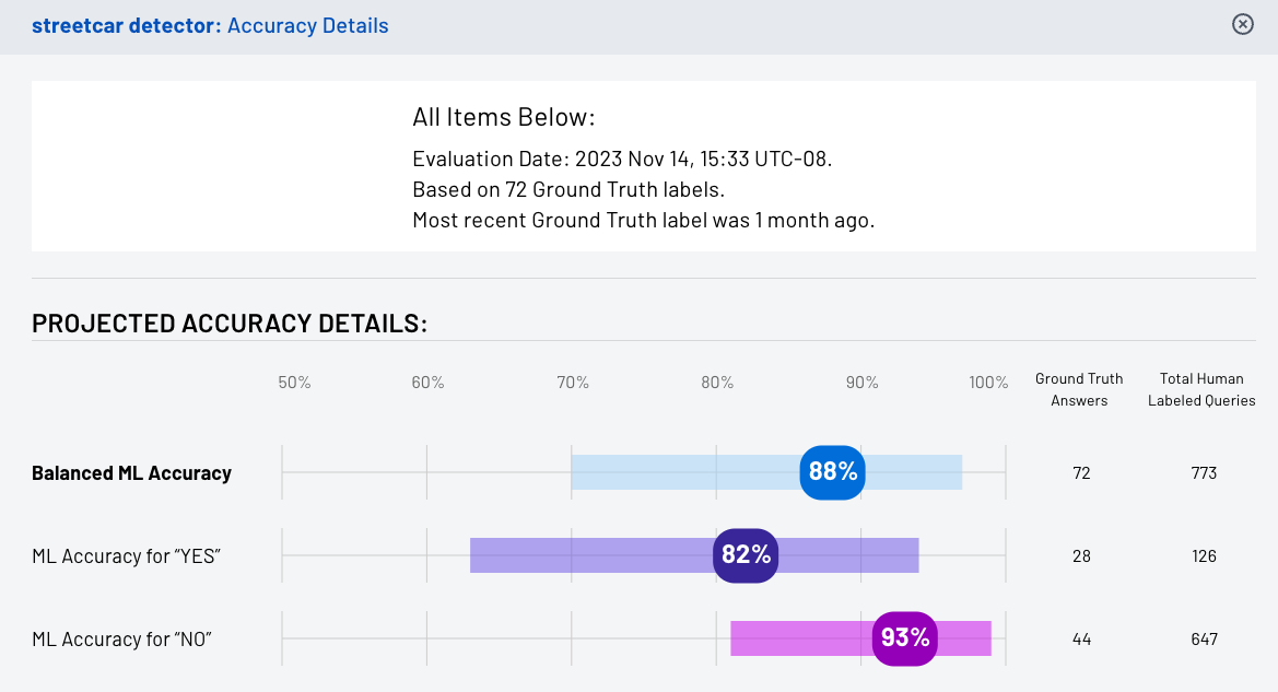
Figure 1: the detector accuracy details view shows balanced accuracy and per-class accuracy with exact 95% confidence intervals

However, we've found that just displaying the balanced accuracy is not informative enough, as we do not always have an ample supply of ground truth labeled images to estimate it from. Ground truth labels are answers to image queries that have been provided by a customer, or customer representative, and are therefore trusted to be correct. With only a few ground truth labels, the estimate of a detector's balanced accuracy may itself be inaccurate. As such, we find it helpful to quantify and display the degree of possible inaccuracy by constructing confidence intervals for balanced accuracy, which brings us to the subject of this blog post!

At Groundlight, we compute and display exact confidence intervals in order to upper and lower bound each detector's balanced accuracy, and thereby convey the amount of precision in the reported metric. The detector's accuracy details view displays these intervals as colored bars surrounding the reported accuracy numbers (see figure 1, above). This blog post describes the mathematics behind how we compute the intervals using the tails of the binomial distribution, and it also strives to provide a healthy amount of intuition for the math.

Unlike the approximate confidence intervals based on the Gaussian distribution, which you may be familiar with, confidence intervals based on the binomial tails are exact, regardless of the number of ground truth labels we have available. Our exposition largely follows Langford, 2005 and we use his "program bound" as a primitive to construct confidence intervals for the balanced accuracy metric.

Background

To estimate and construct confidence intervals for balanced accuracy, we first need to understand how to construct confidence intervals for standard "plain old" accuracy. So we'll start here.

Recall that standard accuracy is just the fraction of predictions a classifier makes which happen to be correct. This sounds simple enough, but to define this fraction rigorously, we actually need to make assumptions. To see why, consider the case that our classifier performs well on daytime images but poorly on nighttime ones. If the stream of images consists mainly of daytime photos, then our classifier's accuracy will be high, but if it's mainly nighttime images, our classifier's accuracy will be low. Or if the stream of images drifts slowly over time from day to nighttime images, our classifier won't even have a single accuracy. Its accuracy will be time-period dependent.

Therefore, a classifier's "true accuracy" is inherently a function of the distribution of examples it's applied to. In practice, we almost never know what this distribution is. In fact, it's something of a mathematical fiction. But it happens to be a useful fiction in so far as it reflects reality, in that it lets us do things like bound the Platonic true accuracy of a classifier and otherwise reason about out-of-sample performance. Consequently, we make the assumption that there exists a distribution over the set of examples that our classifier sees, and that this distribution remains fixed over time.

Let's call the distribution over images that our classifier sees, $D$. Each example in $D$ consists of an image, $x \in \mathcal{X}$, and an associated binary label, $y \in$ { YES, NO }, which is the answer to the query. Let $(x,y) \sim D$ denote the action of sampling an example from $D$. We conceptualize our machine learning classifier as a function, $h$, which maps from the set of images, $\mathcal{X}$, to the set of labels, $\mathcal{Y}$. We say that $h$ correctly classifies an example $(x,y)$ if $h(x) = y$, and that $h$ misclassifies it otherwise.

For now, our goal is to construct a confidence inverval for the true, but unknown, accuracy of $h$. We define this true accuracy as the probability that $h$ correctly classifies an example drawn from $D$:

$$\text{acc}_{D}(h) = \Pr_{(x,y) \sim D}[ \,h(x) = y\, ].$$

The true accuracy is impossible to compute exactly because $D$ is unknown and the universe of images is impossibly large. However, we can estimate it by evaluating $h$ on a finite set of test examples, $S$, which have been drawn i.i.d. from $D$. That is,

$$S = \{ (x_1, y_1), (x_2, y_2), ..., (x_{n}, y_{n}) \}$$

where each $(x_i, y_i) \sim D$ for $i=1,\ldots,n$.

The fraction of images in $S$ that $h$ correctly classifies is called $h$'s empirical accuracy on $S$, and this fraction is computed as

$$\widehat{\text{acc}}_{S}(h) = \frac{1}{n} \sum_{i=1}^n \mathbf{1}[\, h(x_i) = y_i \,].$$

The notation $\mathbf{1}[\, \texttt{condition} \,]$ is shorthand for the indicator function which equals 1 when the $\texttt{condition}$ is true and 0 otherwise. So the formula above just sums the number of examples in $S$ that are correctly classified and then multiplies by 1/n.

The egg-shaped infographic below depicts the scenario of estimating $h$'s true accuracy from its performance on a finite test set. The gray ellipse represents the full distribution of examples, $D$. Each dot corresponds to a single example image, $x$, whose true label, $y$, is represented by the dot's color - red for YES and blue for NO. The classifier, $h$, is represented by the dotted black line. Here, $h$ is the decision rule that classifies all points to the left of the line as should-be YES and all points to the right as should-be-NO. The points with light gray circles around them are the ones that have been sampled to form the test set, $S$.

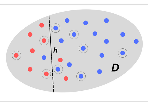
Figure 2: true accuracy can only be estimated from performance on a finite test set. The gray shaded region represents the full distribution. The lightly circled points are examples sampled for the test set.

In this case, our choice of test set, $S$, was unlucky because $h$'s empirical accuracy on $S$ looks great, appearing to be 9/9 = 100%. But evaluating $h$ on the full distribution of examples, $D$, reveals that its true accuracy is much lower, only 24/27 = 89%. If our goal is to rarely be fooled into thinking that $h$'s performance is much better than it really is, then this particular test set was unfortunate in the sense that $h$ performs misleadingly well.

Test Set Accuracy and Coin Flips

It turns out that the problem of determining a classifier's true accuracy from its performance on a finite test set exactly mirrors the problem of determining the bias of a possibly unfair coin after observing some number of flips. In this analogy, the act of classifying an example corresponds to flipping the coin, and the coin landing heads corresponds to the classifier's prediction being correct.

Usefully, the binomial distribution completely characterizes the probability of observing $k$ heads in $N$ independent tosses of a biased coin whose bias, or propensity to land heads, is known to be the probability, $p$, through its probability mass function (PMF), defined as

$$f_{N,p}(k) = {N \choose k} p^k (1 - p)^{N-k}.$$

The cumulative density function (CDF) is the associated function that sums up the PMF probabilities over all outcomes (i.e., number of heads) from 0 through $k$. It tells us the probability of observing $k$ or fewer heads in $N$ independent tosses when the coin's bias is the probability $p$. The CDF is defined as

$$F_{N,p}(k) = \sum_{j = 0}^k f_{N,p}(k).$$

Below we've plotted the PMF (left) and CDF (right) functions for a binomial distribution whose parameters are N=30 and p=0.3.

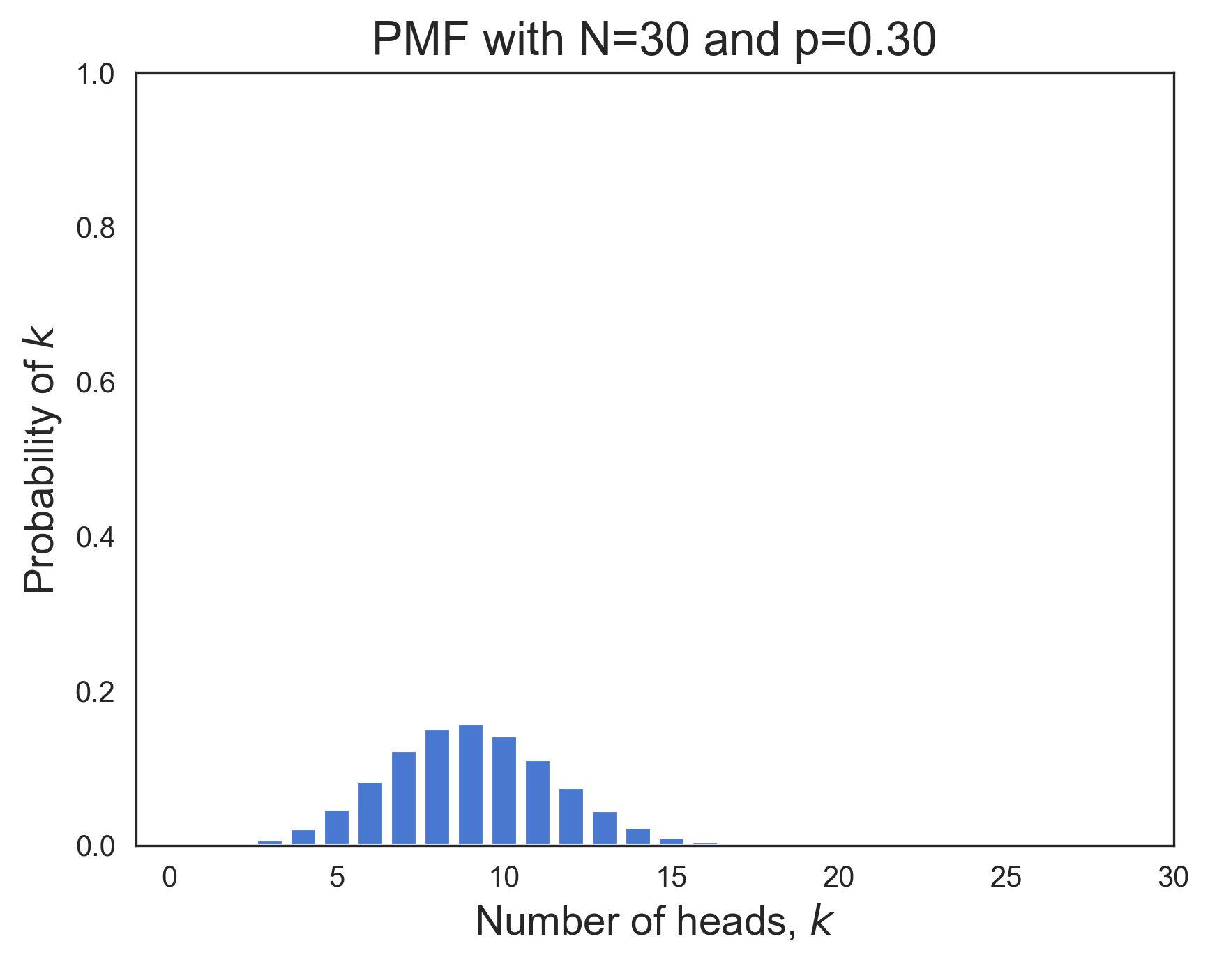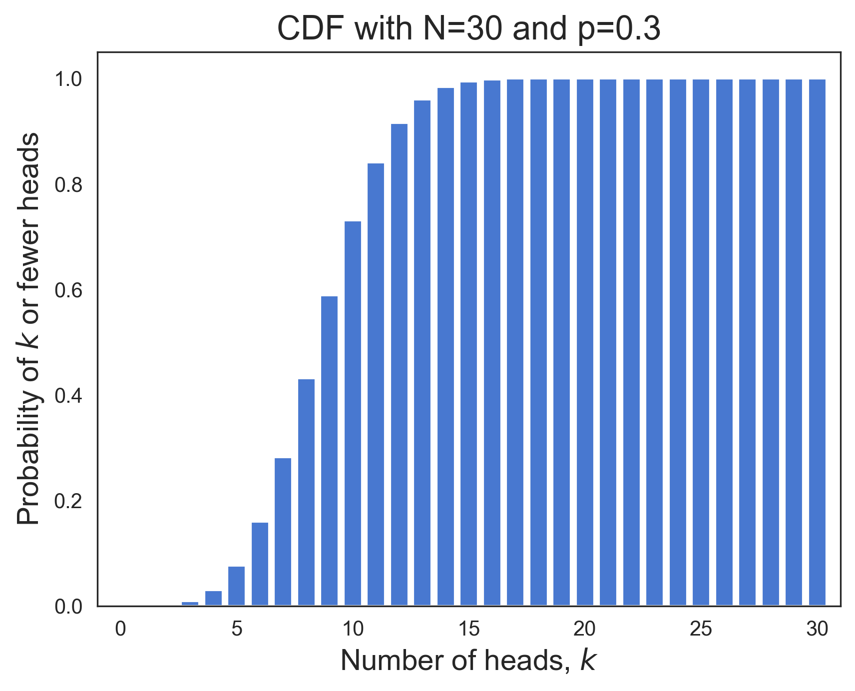The PMF looks like a symmetric "bell curve". Its x-axis is the number of tosses that are heads, $k$. And its y-axis is the probability of observing $k$ heads in $N$ tosses. The CDF plot shows the cumulative sum of the PMF probabilities up through $k$ on its y-axis. The CDF is a monotonically increasing function of $k$. Its value is 1.0 on the right side of the plot since the sum of all PMF probabilities must equal one.

The binomial PMF doesn't always resemble a bell-shaped curve. This is true of the binomial distributions in the two plots below, whose respective bias parameters are p=0.15 and p=0.96.

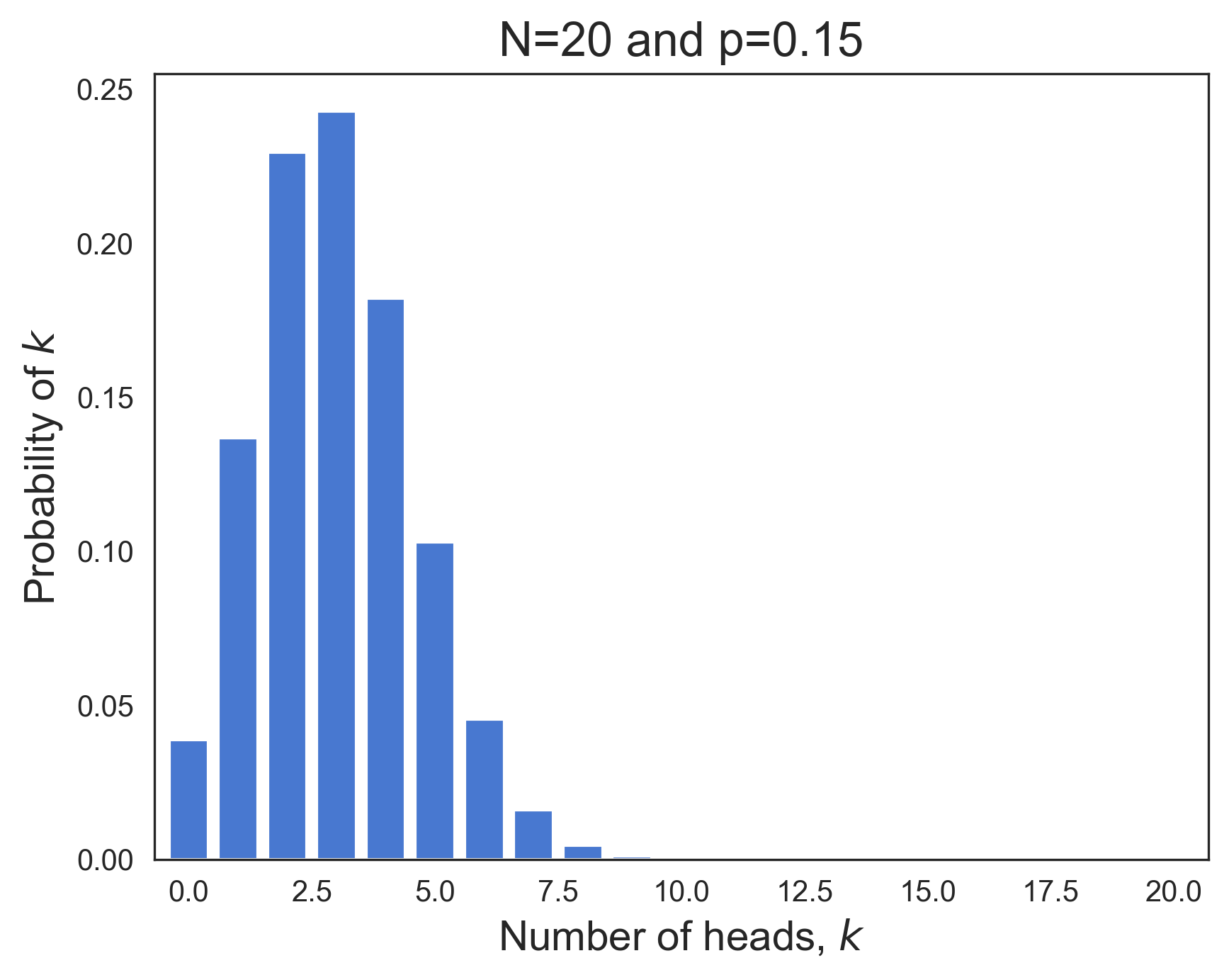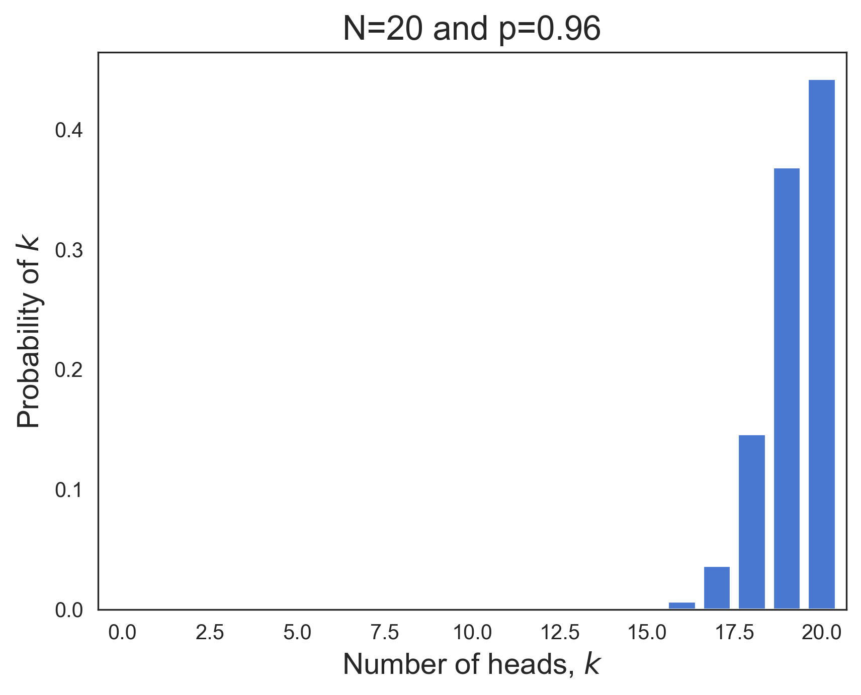Upper Bounding the True Accuracy from Test Set Performance

Now that we've examined the probability of coin tossing and seen how the number of heads from tosses of a biased coin mirrors the number of correctly classified examples in a randomly sampled test set, let's consider the problem of determining an upper bound for the true accuracy of a classifier given its performance on a test set.

Imagine that we've sampled a test set, $S$, from $D$ with 100 examples, and that our classifier, $h$, correctly classified 80 of them. We would like to upper bound $h$'s true accuracy, $\text{acc}_D(h)$, having observed its empirical accuracy, $\widehat{\text{acc}}_S(h)$ = 80/100 = 80%.

Let's start by considering a very naive choice for the upper bound, taking it to equal the empirical accuracy of 80%.

The figure below plots the PMF of a binomial distribution with parameters N=100 and p=0.80. Here, N is the test set size and p corresponds to the true, but unknown, classifier accuracy. The plot shows that if our classifier's true accuracy were in fact 80%, there would be a very good chance of observing an even lower empirical accuracy than what we actually observed. This is reflected in the substantial amount of probability mass lying to the left of the purple vertical line, which is placed at the empirical accuracy point of 80/100 = 80%.

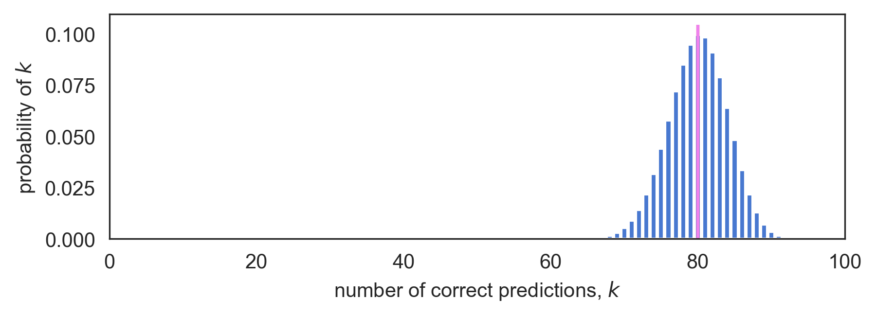
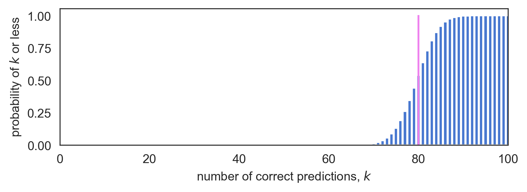
Figure 3: Binomial PMF (top) and CDF (bottom) for N=100 and true accuracy 80.0%. The CDF shows there is a 54% chance of seeing an empirical accuracy of 80% or less.

In fact, the CDF of the binomial tells us that there is a 54% chance of seeing an empirical accuracy of 80% or less when the true accuracy is 80%. And since 54% is fairly good odds, our naive choice of 80% as an upper bound doesn't appear very safe. It would therefore be wise to increase our upper bound if we want it to be an upper bound!

In contrast, the plot below shows that if the true accuracy were a bit higher, say 83%, we would only have a 1 in 4 chance of observing an empirical accuracy less than or equal to our observed accuracy of 80%. Or put differently, roughly a quarter of the test sets we could sample from $D$ would yield an empirical accuracy of 80% or lower if $h$'s true accuracy was 83%. This is shown by the 24.8% probability mass located to the left of the purple line at the 80% empirical accuracy point. The red line is positioned at the hypothesized true accuracy of 83%.

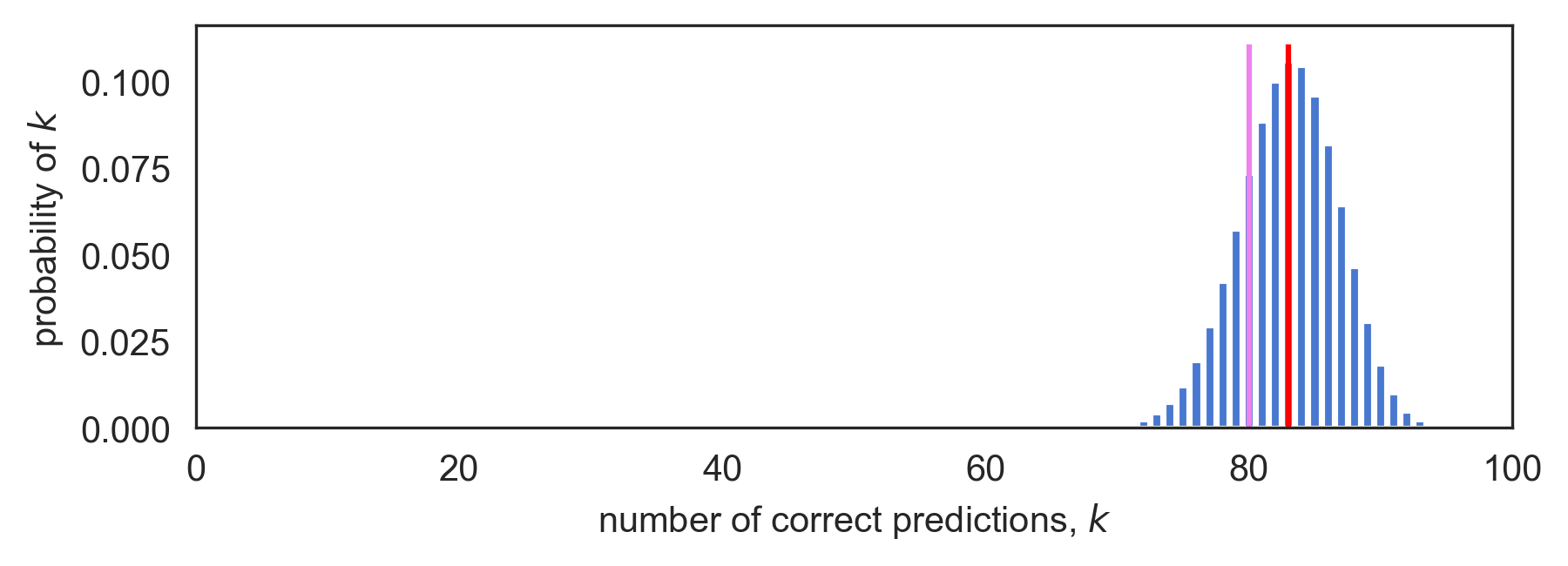
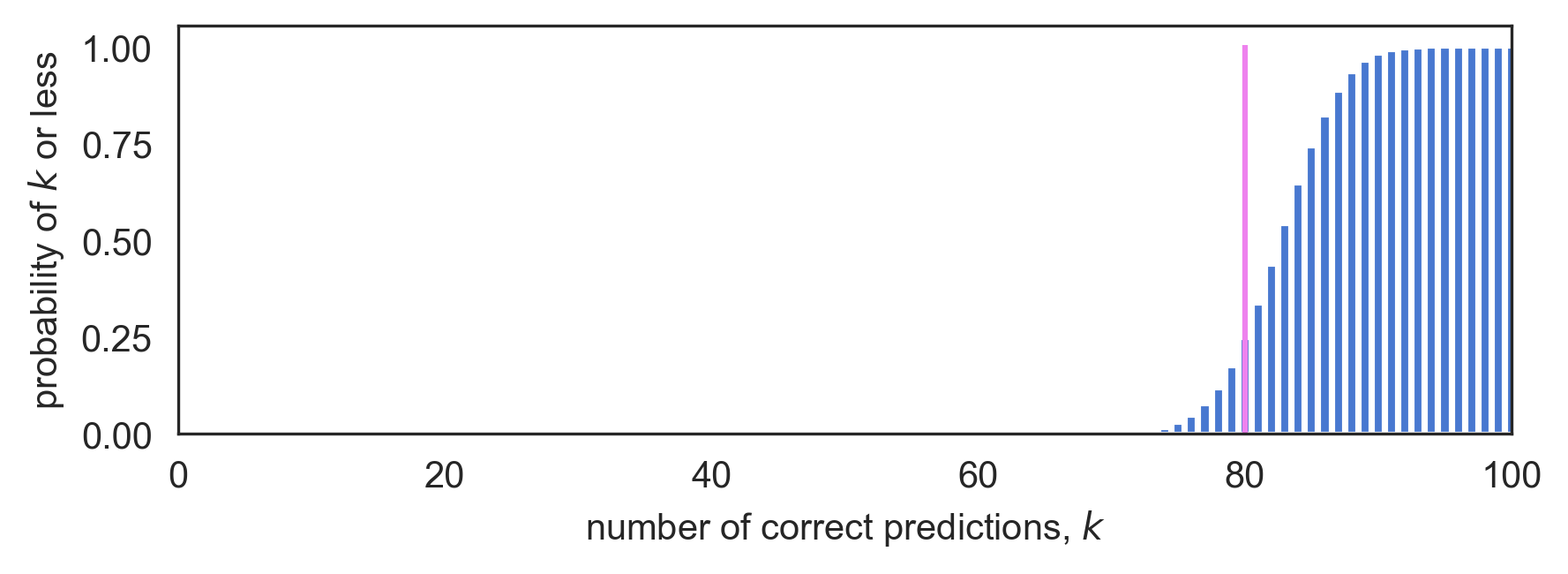
Figure 4: Binomial PMF (top) and CDF (bottom) for N=100 and true accuracy 83.0%. The CDF shows there is a 24.8% chance of seeing an empirical accuracy of 80% or less.

Still, events with one in four odds are quite common, so hypothesizing an even larger true accuracy would be wise if we want to ensure it's not less than the actual true accuracy.

The next plot shows that if the true accuracy were higher still, at 86.3%, the empirical accuracy of 80% or less would be observed on only 5% of sampled test sets. This is evidenced by the even smaller amount of probability mass to the left of the purple line located at the empirical accuracy of 80%. Again, the red line is positioned at the hypothesized true accuracy of 86.3%.

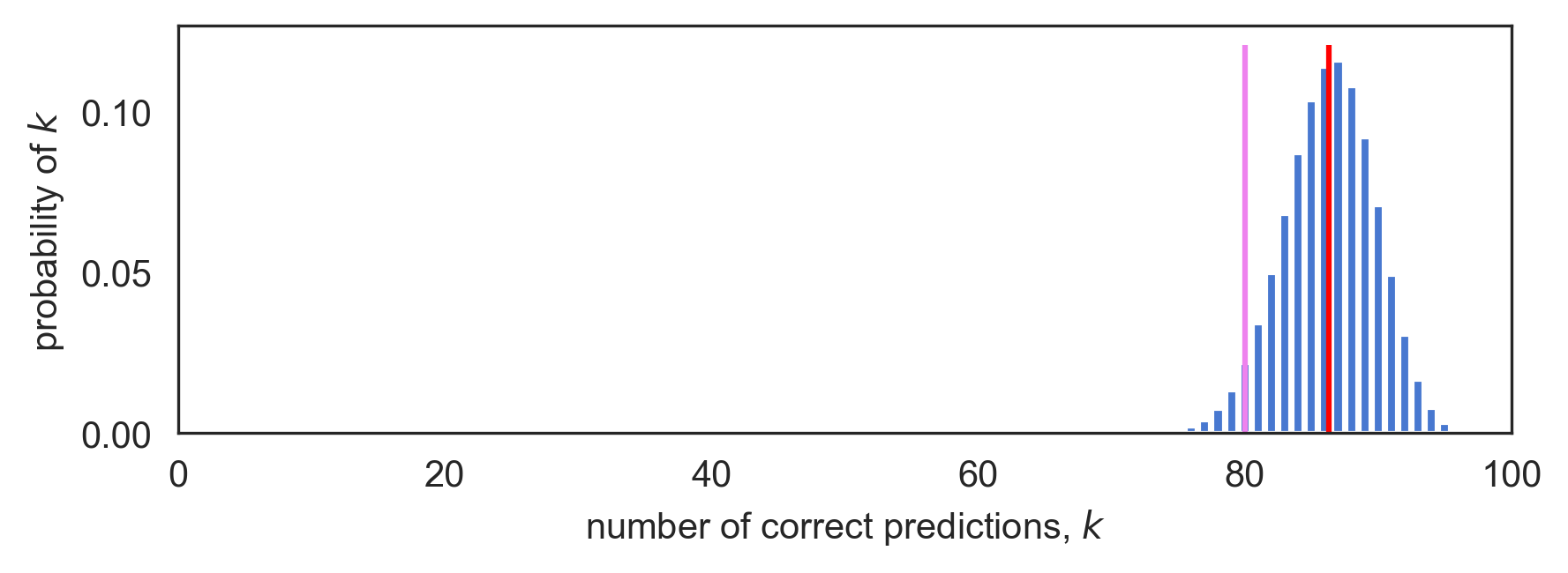
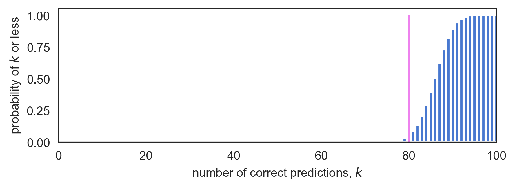
Figure 5: Binomial PMF (top) and CDF (bottom) for N=100 and true accuracy 86.3%. The CDF shows there is a 5% chance of seeing an empirical accuracy of 80% or less.

In other words, if $h$'s true accuracy were 86.3% or greater, we'd observe an empirical accuracy of 80% or lower on just 1 in 20 test sets. Consequently, the hypothesized true accuracy of 86.3% seems like a pretty safe choice for an upper bound.

Constructing a 95% Upper Confidence Bound

The procedure we just outlined, of increasing the hypothesized true accuracy starting from the observed empirical accuracy until exactly 5% of the binomial's probability mass lies to the left of the empirical accuracy, is how we construct an exact 95% upper confidence bound for the true accuracy.

Remarkably, if we apply this procedure many times to find 95% accuracy upper confidence bounds for different ML classifiers at Groundlight, the computed upper bounds will in fact be larger than the respective classifiers' true accuracies in 95% of these encountered cases. This last statement is worth mulling over because it is exactly the right way to think about the guarantees associated with upper confidence bounds.

Restated, a 95% upper confidence bound procedure for the true accuracy is one that produces a quantity greater than the true accuracy 95% of the time.

Exact Upper Confidence Bounds based on the Binomial CDF

So now that we've intuitively described the procedure used to derive exact upper confidence bounds, we give a more formal treatment that will be useful in discussing confidence intervals for balanced accuracy.

First, recall that the binomial's CDF function, $F_{N,p}(k)$, gives the probability of observing $k$ or fewer heads in $N$ tosses of a biased coin whose bias is $p$.

Also, recall in the previous section that we decided to put exactly 5% of the probability mass in the lower tail of the PMF, and this yielded a 95% upper confidence bound. But we could have placed 1% in the lower tail, and doing so would have yielded a 99% upper confidence bound. A 99% upper confidence bound is looser than a 95% upper bound, but it upper bounds the true accuracy on 99% of test sets sampled as opposed to just 95%.

The tightness of the bound versus the fraction of test sets it holds for is a trade off that we get to make referred to as the coverage. We control the coverage through a parameter named $\delta$. Above we had set $\delta$ to 5% which gave us a 1 - $\delta$ = 95% upper confidence bound. But we could have picked some other value for $\delta$.

With $\delta$ understood, we are now ready to give our formal definition of upper confidence bounds. Let $\delta$ be given, $N$ be the number of examples in the test set, $k$ be the number of correctly classified test examples, and $p$ be the true accuracy.

Definition: the 100(1 - $\delta$)% binomial upper confidence bound for $p$ is defined as

$$\bar{p}(N, k, \delta) = \max \{ \, p \,:\, F_{N,p}(k) \ge \delta \,\, \}.$$

In words, $\bar{p}$ is the maximum accuracy for which there exists at least $\delta$ probability mass in the lower tail lying to the left of the observed number of correct classifications for the test set. And this definition exactly mirrors the procedure we used above to find the 95% upper confidence bound. We picked $\bar{p}$ to be the max $p$ such that the CDF $F_{N=100,p}(k=80)$ was at least $\delta$ = 5%.

We can easily implement this definition in code. The binomial CDF is available in python through the scipy.stats module as binom.cdf. And we can use it to find the largest value of $p$ for which $F_{N,p}(k) \ge \delta$. However the CDF isn't directly invertible, so we can't just plug in $\delta$ and get $\bar{p}$ out. Instead we need to search over possible values of $p$ until we find the largest one that satisfies the inequality. This can be done efficiently using the interval bisection method which we implement below.

from scipy.stats import binom

def binomial_upper_bound(N, k, delta):
    """
    Returns a 100*(1 - delta)% upper confidence bound on the accuracy
    of a classifier that correctly classifies k out of N examples.
    """
    def cdf(p):
        return binom.cdf(k, N, p)

    def search(low, high):
        if high - low < 1e-6:
            return low  # we have converged close enough
        mid = (low + high) / 2
        if cdf(mid) >= delta:
            return search(mid, high)
        else:
            return search(low, mid)

    return search(low=k/N, high=1.0)

Lower Confidence Bounds

Referring back to our discussion of coin flips makes it clear how to construct lower bounds for true accuracy. We had likened a correct classification to a biased coin landing heads and we upper bounded the probability of heads based on the observed number of heads.

But we could have used the same math to upper bound the probability of tails. And likening tails to misclassifications lets us upper bound the true error rate. Moreover, the error rate equals one minus the accuracy. And so we immediately get a lower bound on the accuracy by computing an upper bound on the error rate and subtracting it from one.

Again, let $\delta$ be given, $N$ be the number of test examples, $k$ be the number of correctly classified test examples, and let $p$ be the true, but unknown, accuracy.

Definition: the 100(1 - $\delta$)% binomial lower confidence bound for $p$ is defined as

$$\underline{p}(N, k, \delta) = 1 - \max \{ \, p \,:\, F_{N,p}(N - k) \ge \delta \,\, \}.$$

Here $N - k$ is the number of misclassified examples observed in the test set.

Central Confidence Intervals

Now that we know how to derive upper and lower bounds which hold individually at a given confidence level, we can use our understanding to derive upper and lower bounds which hold simultaneously at the given confidence level. To do so, we compute what is called a central confidence interval. A 100$\times$(1 - $\delta$)% central confidence interval is computed by running the upper and lower bound procedures with the adjusted confidence level of 100$\times$(1 - $\delta$/2)%.

For example, if we want to compute a 95% central confidence interval, we compute 97.5% lower and upper confidence bounds. This places $\delta$/2 = 2.5% probability mass in each tail, thereby providing 95% coverage in the central region.

Pictorially below, you can see that the 95% central confidence interval (top row) produces wider bounds than just using the 95% lower and upper confidence bounds separately (bottom row). The looser bounds are unfortunate. But naively computing the lower and upper bounds at the original confidence level of 95% sacrifices coverage due to multiple testing.

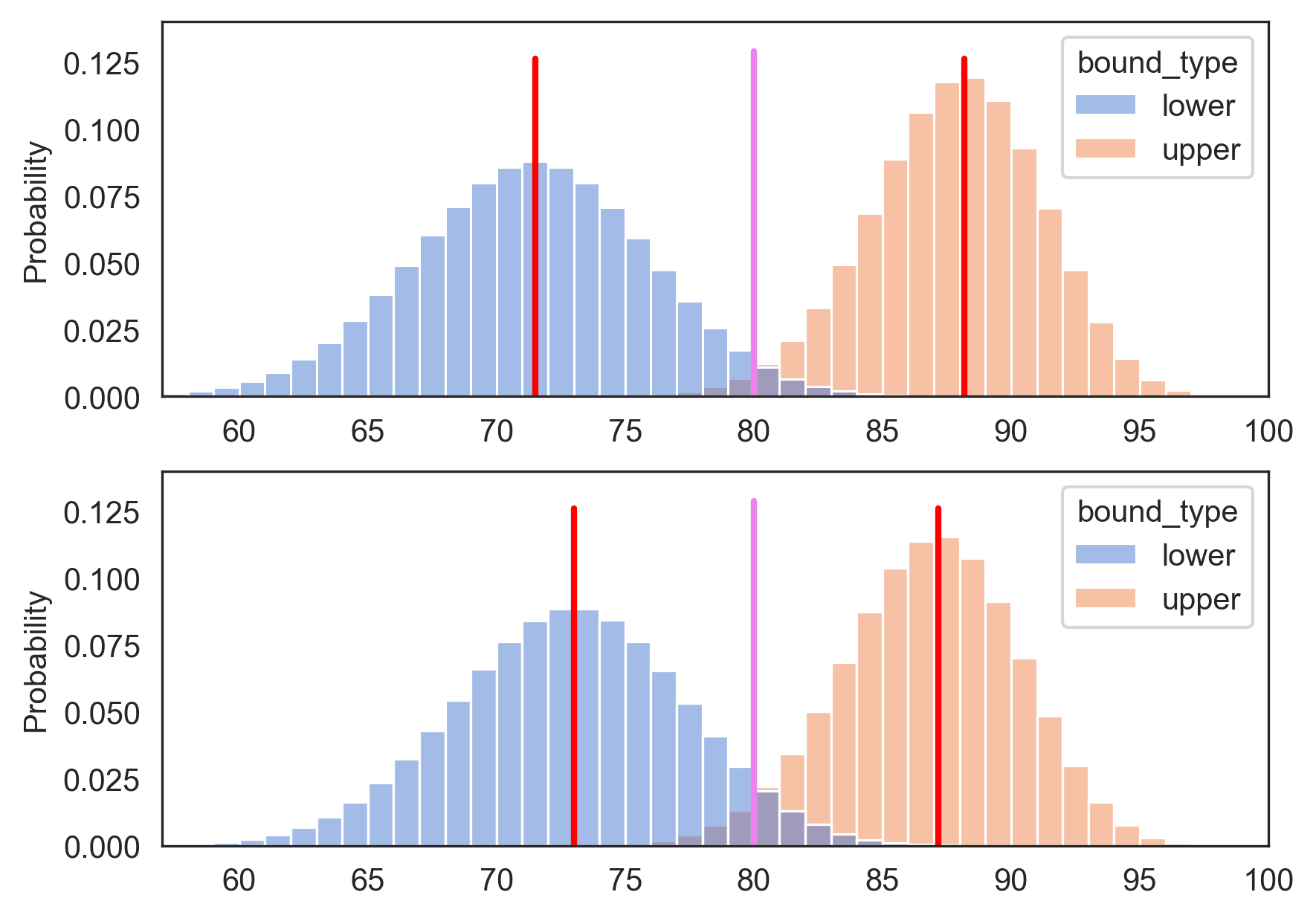
Figure 6: central confidence intervals produce wider bounds to correct for multiple testing

In the next section, where we compute central confidence intervals for balanced accuracy, we will have to do even more to correct for multiple testing.

Confidence Bounds for Balanced Accuracy

Recall that the balanced accuracy for a binary classifier is the mean of its accuracy on examples from the positive class and its accuracy on examples from the negative class.

To define what we mean by the "true balanced accuracy", we need to define appropriate distributions over examples from each class. To do so, we decompose $D$ into separate class conditional distributions, $D^+$ and $D^-$, where

$$\Pr\left\{ (x,y) \sim D^+ \right\} = \Pr\left\{ (x,y) \sim D \mid y = +1 \right\},$$ $$\Pr\left\{ (x,y) \sim D^- \right\} = \Pr\left\{ (x,y) \sim D \mid y = -1 \right\}.$$

The positive and negative true accuracies are defined with respect to each of these class specific distributions:

$$\text{acc}^+(h) = E_{(x,y) \sim D^+} \, \mathbf{1}[ h(x_i) = y_i ],$$ $$\text{acc}^-(h) = E_{(x,y) \sim D^-} \, \mathbf{1}[ h(x_i) = y_i ].$$

The true balanced accuracy is then defined as the average of these,

$$\text{acc}_\text{bal}(h) = \frac{\text{acc}^+(h) + \text{acc}^-(h)}{2}.$$

Constructing the Bound for Balanced Accuracy

With the above definitions in hand, we can now bound the balanced accuracy of our classifier based on its performance on a test set. Let $S$ be the test set, and let

• $N^+$ denote the number of positive examples in $S$
• $N^-$ denote the number of negative examples in $S$
• $k^+$ denote the number of positive examples in $S$ that $h$ correctly classified
• $k^-$ denote the number of negative examples in $S$ that $h$ correctly classified

From these quantities, we can find lower and upper bounds for the positive and negative accuracies based on the binomial CDF.

Denote these lower and upper bounds on positive and negative accuracy as

$$\underline{\text{acc}^+}(h) ,~~ \overline{\text{acc}^+}(h) ,~~ \underline{\text{acc}^-}(h) ,~~ \overline{\text{acc}^-}(h).$$

To find a 100(1 - $\delta$)% confidence interval for the $\text{acc}_\text{bal}(h)$, we first compute the quantities

$$\underline{\text{acc}^+}(h) = \underline{p}(N^+, k^+, \delta/4) ~~ \text{ and } ~~ \overline{\text{acc}^+}(h) = \overline{p}(N^+, k^+, \delta/4)$$ $$\underline{\text{acc}^-}(h) = \underline{p}(N^-, k^-, \delta/4) ~~ \text{ and } ~~ \overline{\text{acc}^-}(h) = \overline{p}(N^-, k^-, \delta/4)$$

Importantly, we've used an adjusted delta value of $\delta/4$ to account for mulitple testing. That is, if we desire our overall coverage to be (1 - $\delta$) = 95%, we run our individual bounding procedures with the substituted delta value of $\delta/4 = 1.25\%$.

The reason why is as follows. By construction, each of the four bounds will fail to hold with probability $\delta/4$. The union bound in appendix A tells us that the probability of at least one of these four bounds failing is no greater than the sum of the probabilities that each fails. Summing up the failure probabilities for all four bounds, the probability that at least one bound fails is therefore no greater than $4\cdot(\delta/4) = \delta$. Thus the probability that none of the bounds fails is at least 1 - $\delta$, giving us the desired level of coverage.

Last, we obtain our exact lower and upper bounds for balanced accuracy by averaging the respective lower and upper bounds for the positive and negative class accuracies:

$$\underline{\text{acc}_\text{bal}}(h) = (1/2) \left( \underline{\text{acc}^+}(h) + \underline{\text{acc}^-}(h) \right)$$ $$\overline{\text{acc}_\text{bal}}(h) = (1/2) \left( \overline{\text{acc}^+}(h) + \overline{\text{acc}^-}(h) \right)$$

Pictorially below, we can see how the averaged lower and upper bounds contain the true balanced accuracy.

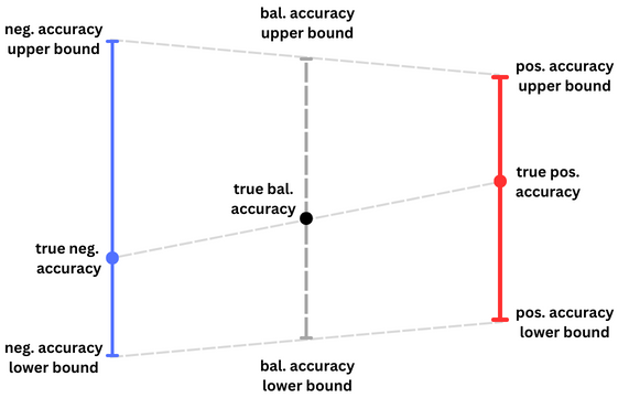
Figure 7: the balanced accuracy is bounded by the respective averages of the lower and upper bounds

Comparison with intervals based on the Normal approximation

The main benefit of using bounds derived from the binomial CDF is that they are exact and always contain the true accuracy the desired fraction of the time.

Let's compare this with the commonly used bound obtained by approximating the binomial PMF with a normal distribution. The motivation for the normal approximation comes from the central limit theorem, which states that for a binomial distribution with parameters $N$ and $p$, the distribution of the empirical accuracy, $\hat{p} = k/N$, converges to a normal distribution as the sample size, $N$, goes to infinity,

$$\hat{p} \stackrel{d}{\longrightarrow} \mathcal{N}\left(p, \frac{p(1-p)}{N}\right).$$

This motivates the use of the traditional two-standard deviation confidence interval in which one reports

$$\Pr\left\{ | p - \hat{p} | \le 1.96 \,\hat{\sigma} \right\} \ge 95\% ~ ~ ~ \text{where} ~ ~ ~ \hat{\sigma} = \sqrt{ \frac{ \hat{p}(1-\hat{p}) }{N} }.$$

But it's well known that the normal distribution poorly approximates the sampling distribution of $\hat{p}$ when $p$ is close to zero or one. For instance, if we observe zero errors on the test set, then $\hat{p}$ will equal 1.0 (i.e., 100% empirical accuracy), and the sample standard deviation, $\hat{\sigma}$, will equal zero. The estimated lower bound will therefore be equal to the empirical accuracy of 100%, which is clearly unbelievable.

And since we train classifiers to have as close to 100% accuracy as possible, the regime in which $p$ is close to one is of major interest. Thus, exact confidence intervals based on the binomial CDF are both more accurate and practically useful than those based on the normal approximation.

Conclusion

At Groundlight, we've put a lot of thought and effort into assessing the performance of our customers' ML models so they can easily understand how their detectors are performing. This includes the use of balanced accuracy as the summary performance metric and exact confidence intervals to convey the precision of the reported metric.

Here we've provided a detailed tour of the methods we use to estimate confidence intervals around balanced accuracy. The estimated intervals are exact in that they possess the stated coverage, no matter how many ground truth labeled examples are available for testing. Our aim in this post has been to provide a better understanding of the metrics we display, how to interpret them, and how they're derived. We hope we've succeeded! If you are interested in reading more about these topics, see the references and brief appendices below.

References

[Langford, 2005] Tutorial on Practical Prediction Theory for Classification. Journal of Machine Learning Research 6 (2005) 273–306.

[Brodersen et al., 2010] The balanced accuracy and its posterior distribution. Proceedings of the 20th International Conference on Pattern Recognition, 3121-24.

Appendix A - the union bound

Recall that the union bound states that for a collection of events, $A_1, A_2, \ldots, A_n$, the probability that at least one of them occurs is less than the sum of the probabilities that each of them occurs: $\Pr\left\{ \cup_{i=1}^n A_i \right\} \le \sum_{i=1}^n \Pr(A_i).$

Pictorially, the union bound is understood from the image below which shows that area of the union of the regions is no greater than the sum of the regions' areas.

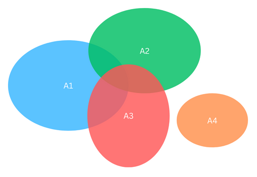
Figure 8: Visualizing the union bound. The area of each region $A_i$ corresponds to the probability that event $A_i$ occurs. The sum of the total covered area must be less than the sum of the individual areas.

Appendix B - interpretation of confidence intervals

The semantics around frequentist confidence intervals is subtle and confusing. The construction of a 95% upper confidence bound does NOT imply there is a 95% probability that the true accuracy is less than the bound. It only guarantees that the true accuracy is less than the upper bound in at least 95% of the cases that we run the the upper confidence bounding procedure (assuming we run the procedure many many times). For each individual case, however, the true accuracy is either greater than or less than the bound. And thus, for each case, the probability that the true accuracy is less than the bound equals either 0 or 1, we just don't know which.

If you instead desire more conditional semantics, you need to use Bayesian credible intervals. See Brodersen et al., 2010 for a nice derivation of credible intervals for balanced accuracy.